Your New Go-To for Time-Sequence Information Visualization

Introducing KitikiPlot, a Python library designed for visualizing sequential and time-series categorical “Sliding Window” patterns. This progressive instrument is designed to empower knowledge practitioners throughout numerous fields, together with genomics, air high quality monitoring, and climate forecasting to uncover insights with enhanced readability and precision. Designed with simplicity and flexibility, it integrates seamlessly with Python’s knowledge ecosystem whereas providing visually interesting outputs for sample recognition. Let’s discover its potential, and rework the best way of analyzing categorical sequences.

Studying Aims

• Perceive the KitikiPlot sliding window visualization approach for sequential and time-series categorical knowledge.
• Discover its parameters to tailor visualizations for particular datasets and functions.
• Apply KitikiPlot throughout numerous domains, together with genomics, climate evaluation, and air high quality monitoring.
• Develop proficiency in visualizing complicated knowledge patterns utilizing Python and Matplotlib.
• Acknowledge the importance of visible readability in categorical knowledge evaluation to reinforce decision-making processes.

This text was revealed as part of the Information Science Blogathon.

KitikiPlot: Simplify Advanced Information Visualization

KitikiPlot is a strong visualization instrument designed to simplify complicated knowledge evaluation, particularly for functions like sliding window graphs and dynamic knowledge illustration. It affords flexibility, vibrant visualizations, and seamless integration with Python, making it perfect for domains reminiscent of genomics, air high quality monitoring, and climate forecasting. With its customizable options, KitikiPlot transforms uncooked knowledge into impactful visuals effortlessly.

• KitikiPlot is a Python library for visualizing sequential and time-series categorical “Sliding Window” knowledge.
• The time period ‘kitiki‘(కిటికీ) means ‘window‘ in Telugu.

Key Options

• Sliding Window: The visible illustration consists of a number of rectangular bars, every similar to knowledge from a particular sliding window.
• Body: Every bar is split into a number of rectangular cells referred to as “Frames.” These frames are organized side-by-side, every representing a price from the sequential categorical knowledge.
• Customization Choices: Customers can customise home windows extensively, together with choices for shade maps, hatching patterns, and alignments.
• Versatile Labeling: The library permits customers to regulate labels, titles, ticks, and legends in line with their preferences.

Getting Began: Your First Steps with KitikiPlot

Dive into the world of KitikiPlot with this quick-start information. From set up to your first visualization, we’ll stroll you thru each step to make your knowledge shine.

Set up KitikiPlot utilizing pip

pip set up kitikiplot

Import “kitikiplot”

import pandas as pd
from kitikiplot import KitikiPlot

Load the dataframe

Thought-about the information body ‘weatherHistory.csv’ from https://www.kaggle.com/datasets/muthuj7/weather-dataset.

df= pd.read_csv( PATH_TO_CSV_FILE )
print("Form: ", df.form)
df= df.iloc[45:65, :]
print("Form: ", df.form)
df.head(3)

ktk= KitikiPlot( knowledge= df["Summary"].values.tolist() )
ktk.plot( ) 

Understanding KitikiPlot Parameters

To totally leverage the ability of KitikiPlot, it’s important to know the varied parameters that management how your knowledge is visualized. These parameters mean you can customise features reminiscent of window dimension, step intervals, and different settings, making certain your visualizations are tailor-made to your particular wants. On this part, we’ll break down key parameters like stride and window_length that can assist you fine-tune your plots for optimum outcomes.

stride : int (elective)

• The variety of components to maneuver the window after every iteration when changing a listing to a DataFrame.
• Default is 1.

index= 0
ktk= KitikiPlot( knowledge= df["Summary"].values.tolist(), stride= 2 )
ktk.plot( cell_width= 2, transpose= True )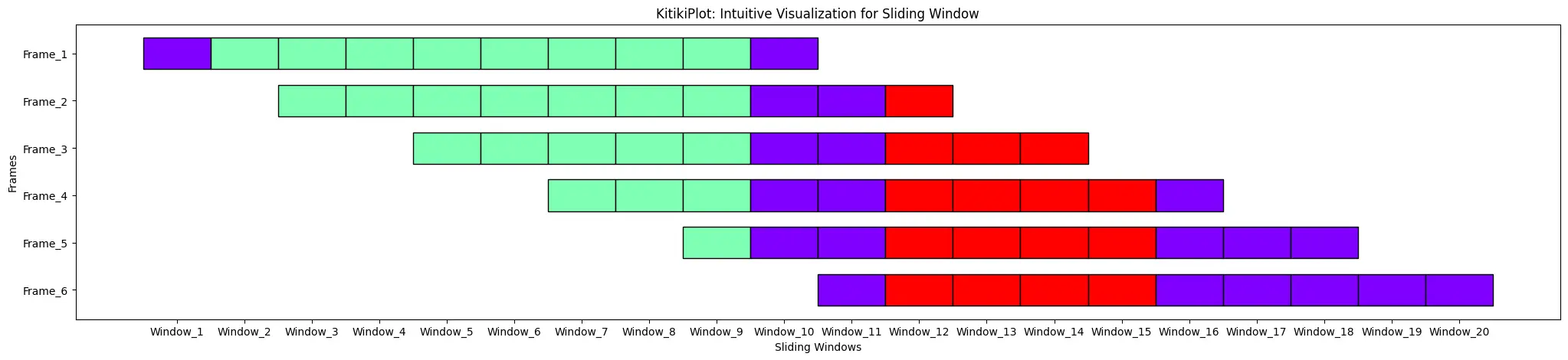

window_length : int (elective)

• The size of every window when changing a listing to a DataFrame.
• Default is 10.

index= 0

ktk= KitikiPlot( knowledge= df["Summary"].values.tolist(), window_length= 5 )

ktk.plot( transpose= True,
          xtick_prefix= "Body",
          ytick_prefix= "Window",
          cell_width= 2 )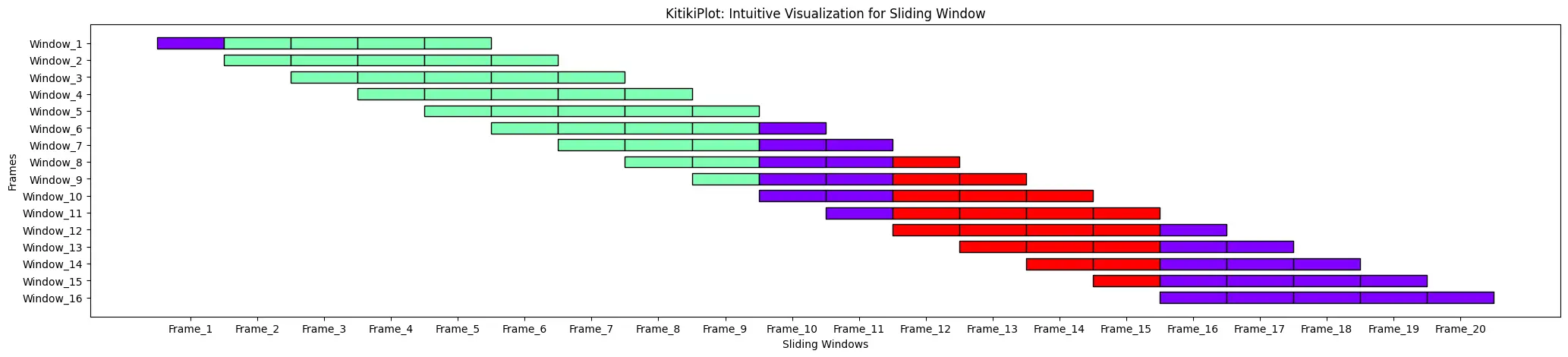   

figsize : tuple (elective)

• The scale of the determine (width, top).
• Default is (25, 5).

ktk= KitikiPlot( knowledge= df["Summary"].values.tolist() )
ktk.plot( figsize= (20, 8) )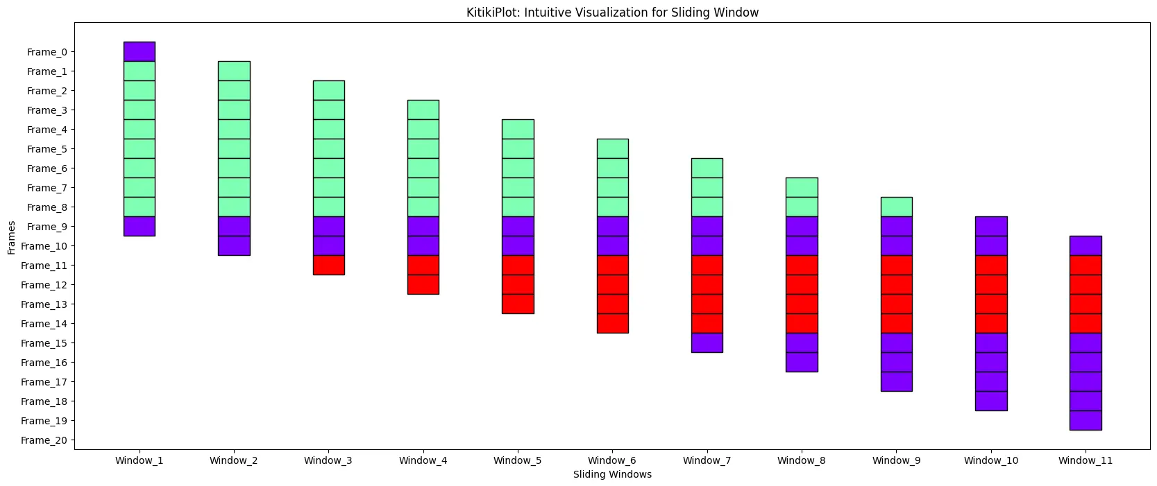

cell_width : float

• The width of every cell within the grid.
• Default is 0.5.

ktk= KitikiPlot( knowledge= df["Summary"].values.tolist() )
ktk.plot( cell_width= 2 )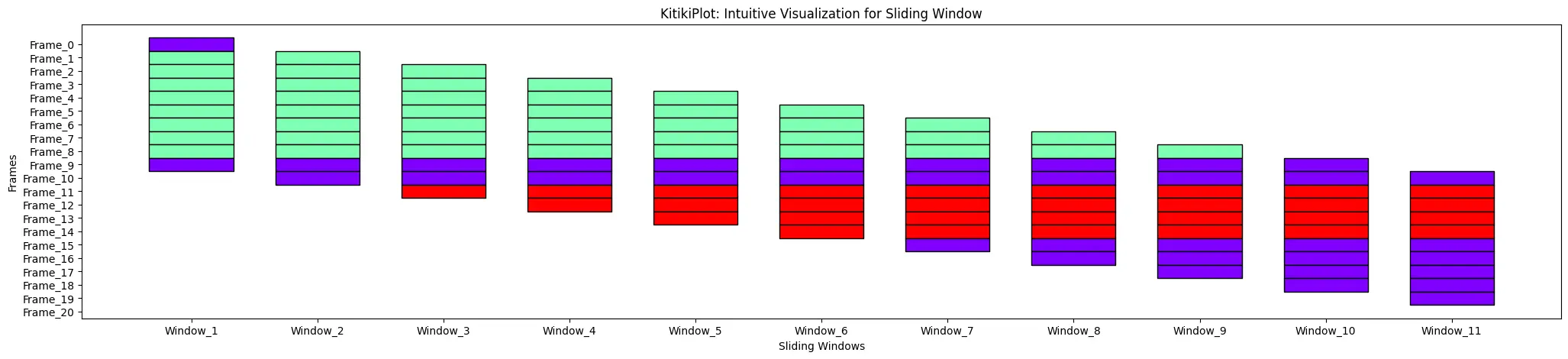

cell_height : float

• The peak of every cell within the grid.
• Default is 2.0.

ktk= KitikiPlot( knowledge= df["Summary"].values.tolist() )
ktk.plot( cell_height= 3 )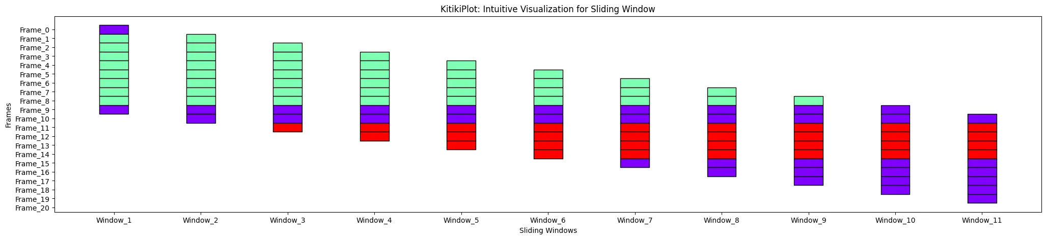

transpose : bool (elective)

• A flag indicating whether or not to transpose the KitikiPlot.
• Default is False.

ktk= KitikiPlot( knowledge= df["Summary"].values.tolist() )
ktk.plot( transpose= False )

ktk= KitikiPlot( knowledge= df["Summary"].values.tolist() )
ktk.plot( 
            cell_width= 2,
            transpose= True,
            xtick_prefix= "Body",
            ytick_prefix= "Window",
            xlabel= "Frames",
            ylabel= "Sliding_Windows" )

window_gap : float

• The hole between cells within the grid.
• Default is 1.0.

ktk= KitikiPlot( knowledge= df["Summary"].values.tolist() )
ktk.plot( window_gap= 3 )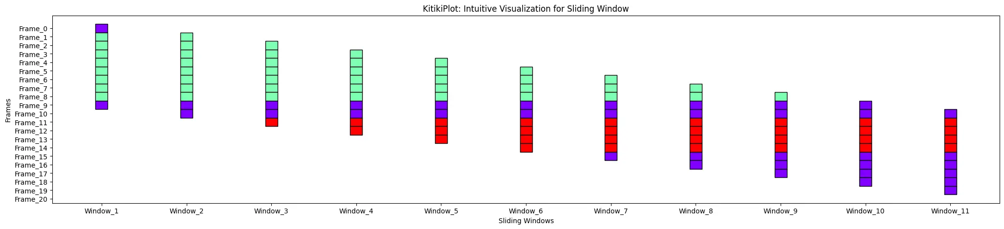

window_range : str or tuple (elective)

• The vary of home windows to show.
• Use “all” to indicate all home windows or specify a tuple (start_index, end_index).
• Default is “all”.

ktk= KitikiPlot( knowledge= df["Summary"].values.tolist() )
ktk.plot( window_range= "all" )

ktk= KitikiPlot( knowledge= df["Summary"].values.tolist() )
ktk.plot( window_range= (3,8) )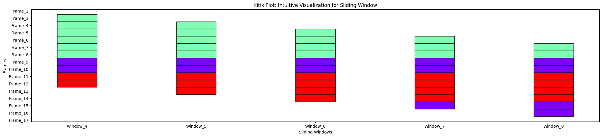

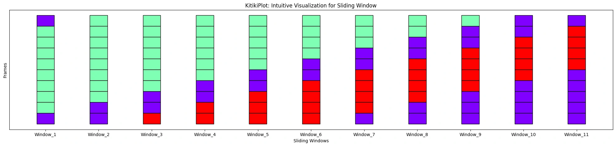
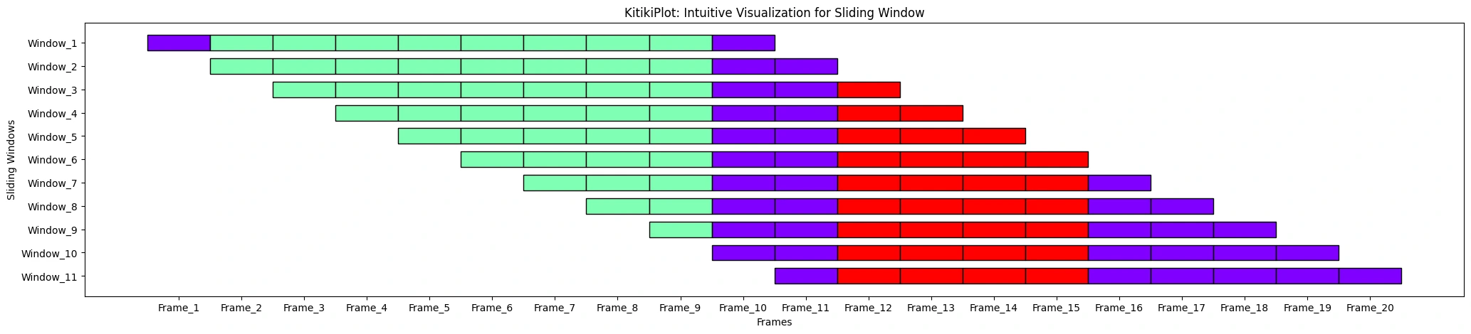
align : bool

• A flag indicating whether or not to shift consecutive bars vertically (if transpose= False), andhorizontally(if transpose= True) by stride worth.
• Default is True.

ktk= KitikiPlot( knowledge= df["Summary"].values.tolist() )
ktk.plot( align= True )

ktk.plot( 
         align= False,
         display_yticks= False # Show no yticks
        )

ktk.plot( 
         cell_width= 2, 
         align= True, 
         transpose= True, 
         xlabel= "Frames",
         ylabel= "Sliding Home windows",
         xtick_prefix= "Body",
         ytick_prefix= "Window"
        )

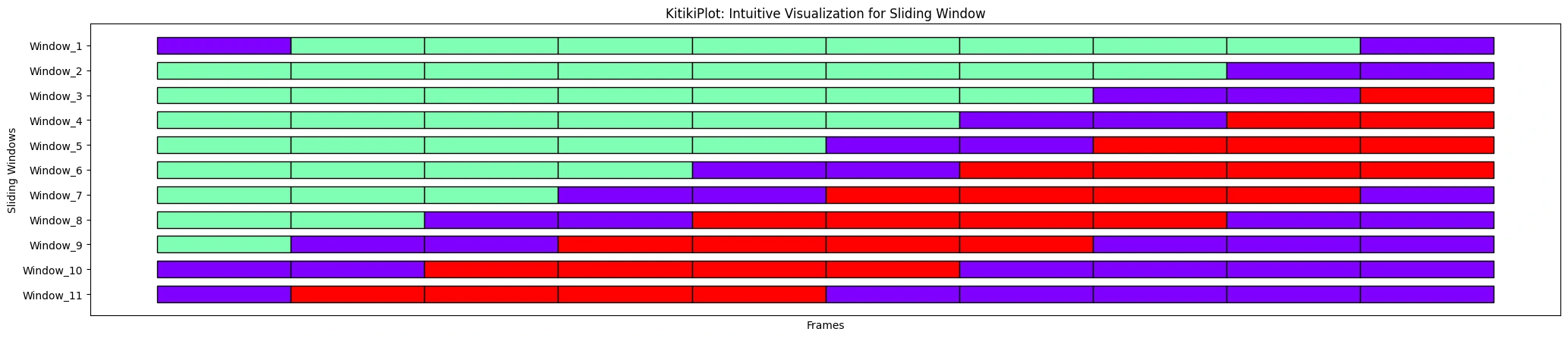
ktk.plot( 
         cell_width= 2, 
         align= False, 
         transpose= True,
         xlabel= "Frames",
         ylabel= "Sliding Home windows",
         ytick_prefix= "Window",
         display_xticks= False 
        )

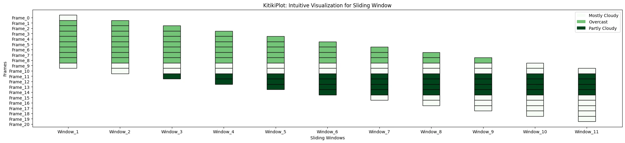
cmap : str or dict

• If a string, it ought to be a colormap identify to generate colours.
• If a dictionary, it ought to map distinctive values to particular colours.
• Default is ‘rainbow’.

ktk= KitikiPlot( knowledge= df["Summary"].values.tolist() )
ktk.plot( 
          cmap= "Greens",
          display_legend= True
        )

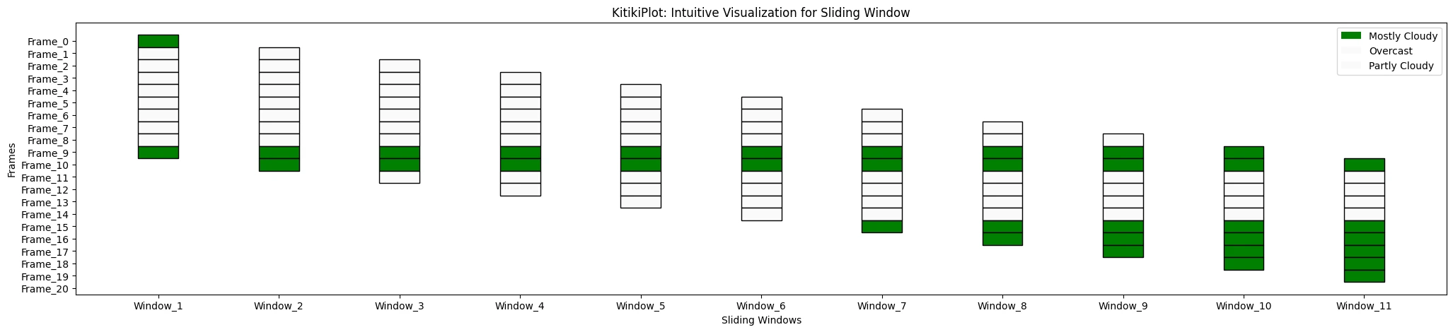
ktk.plot( 
          cmap= {"Largely Cloudy": "Inexperienced"},
          display_legend= True
        )

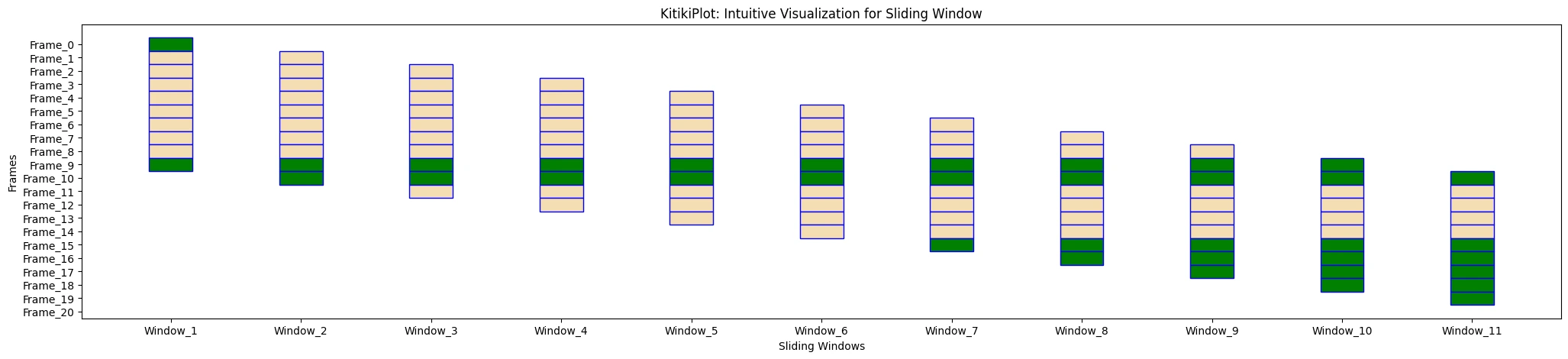
edge_color : str

• The colour to make use of for the sides of the rectangle.
• Default is ‘#000000’.

ktk.plot( 
          cmap= {"Largely Cloudy": "Inexperienced"},
          fallback_color= "wheat",
          edge_color= "blue",
        )

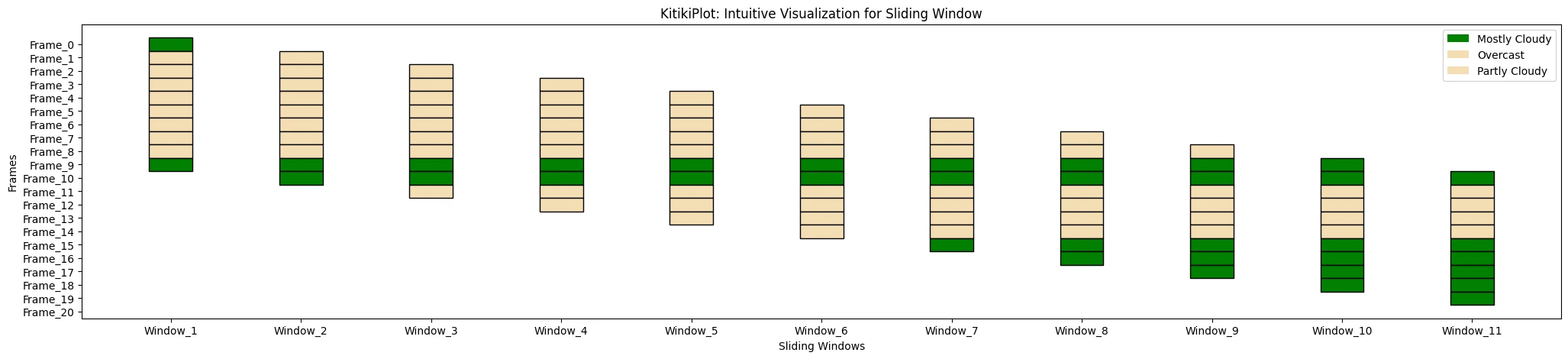
fallback_color : str

• The colour to make use of as fallback if no particular shade is assigned.
• Default is ‘#FAFAFA’.

ktk.plot( 
          cmap= {"Largely Cloudy": "Inexperienced"},
          fallback_color= "wheat",
          display_legend= True
        )

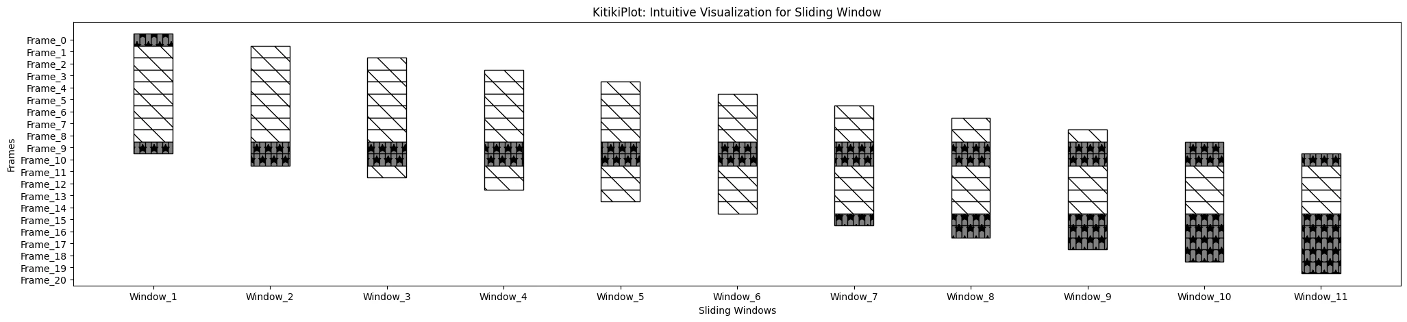
hmap : dict

• A dictionary mapping distinctive values to their corresponding hatch patterns.
• Default is ‘{}’.

ktk= KitikiPlot( knowledge= df["Summary"].values.tolist() )
ktk.plot( 
          cmap= {"Largely Cloudy": "gray"},
          fallback_color= "white",
          hmap= *,
          display_hatch= True
        )

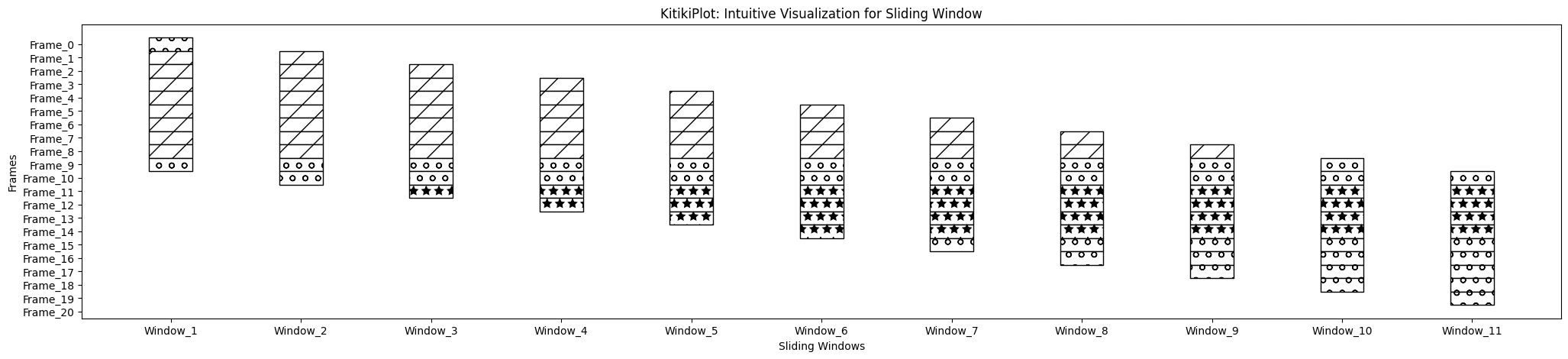
fallback_hatch : str

• The hatch sample to make use of as fallback if no particular hatch is assigned.
• Default is ‘” “‘ (string with single area).

ktk= KitikiPlot( knowledge= df["Summary"].values.tolist() )
ktk.plot( 
          cmap= {"Largely Cloudy": "gray"},
          fallback_color= "white",
          hmap= *,
          fallback_hatch= "",
          display_hatch= True
        )

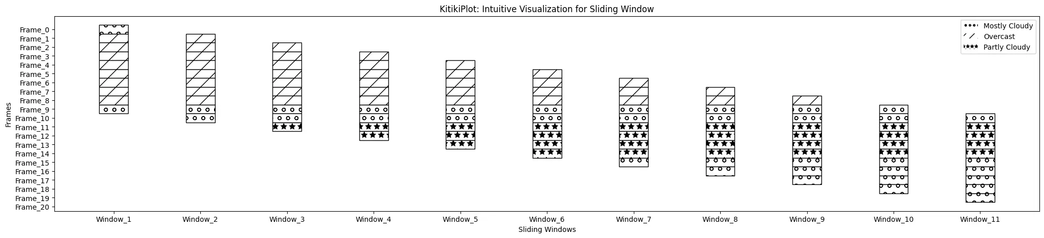
display_hatch : bool

• A flag indicating whether or not to show hatch patterns on cells.
• Default is False.

ktk= KitikiPlot( knowledge= df["Summary"].values.tolist() )

ktk.plot( 
          cmap= {"Largely Cloudy": "#ffffff"},
          fallback_color= "white",
          display_hatch= True
        )

xlabel : str (elective)

• Label for the x-axis.
• Default is “Sliding Home windows”.

ktk= KitikiPlot( knowledge= df["Summary"].values.tolist() )
ktk.plot( xlabel= "Statement Window" )

ylabel : str (elective)

• Label for the y-axis.
• Default is “Frames”.

ktk= KitikiPlot( knowledge= df["Summary"].values.tolist() )
ktk.plot( ylabel= "Body ID" )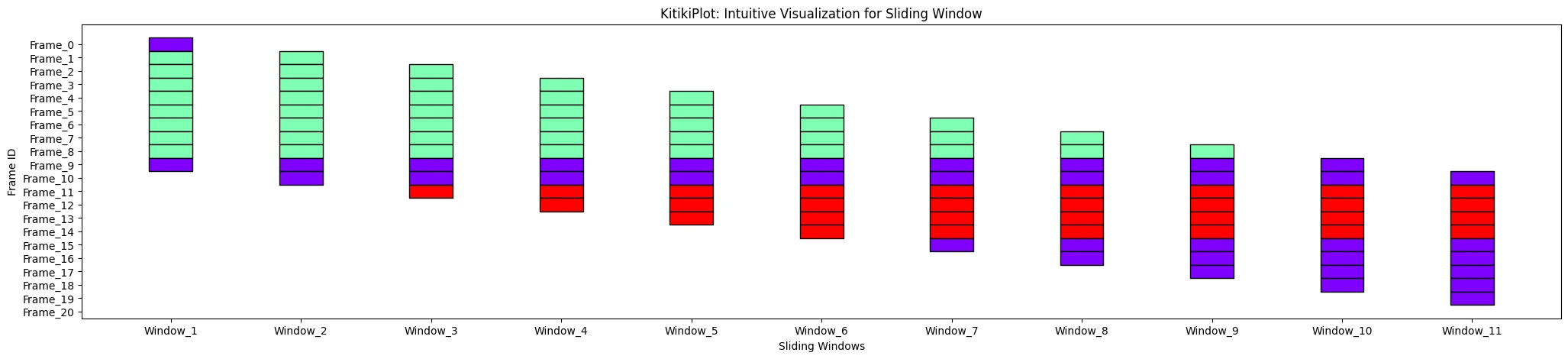

display_xticks : bool (elective)

• A flag indicating whether or not to show xticks.
• Default is True.

ktk= KitikiPlot( knowledge= df["Summary"].values.tolist() )
ktk.plot( display_xticks= False )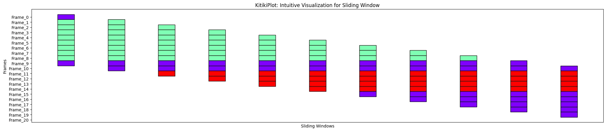

display_yticks : bool (elective)

• A flag indicating whether or not to show yticks
• Default is True

ktk= KitikiPlot( knowledge= df["Summary"].values.tolist() )
ktk.plot( display_yticks= False )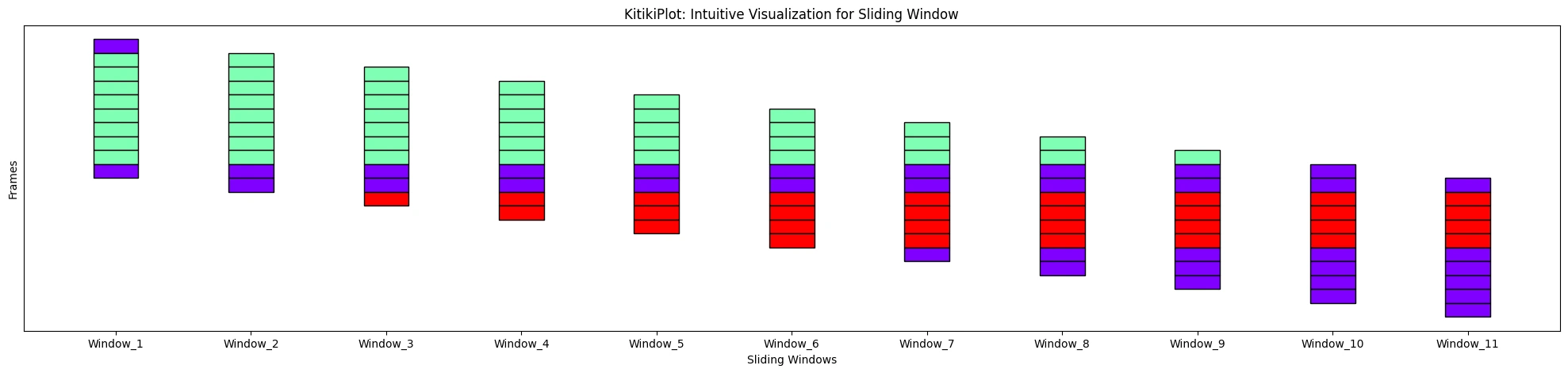

xtick_prefix : str (elective)

• Prefix for x-axis tick labels.
• Default is “Window”.

ktk= KitikiPlot( knowledge= df["Summary"].values.tolist() )
ktk.plot( xtick_prefix= "Statement" )

ytick_prefix : str (elective)

• Prefix for y-axis tick labels.
• Default is “Body”.

ktk= KitikiPlot( knowledge= df["Summary"].values.tolist() )
ktk.plot( ytick_prefix= "Time" )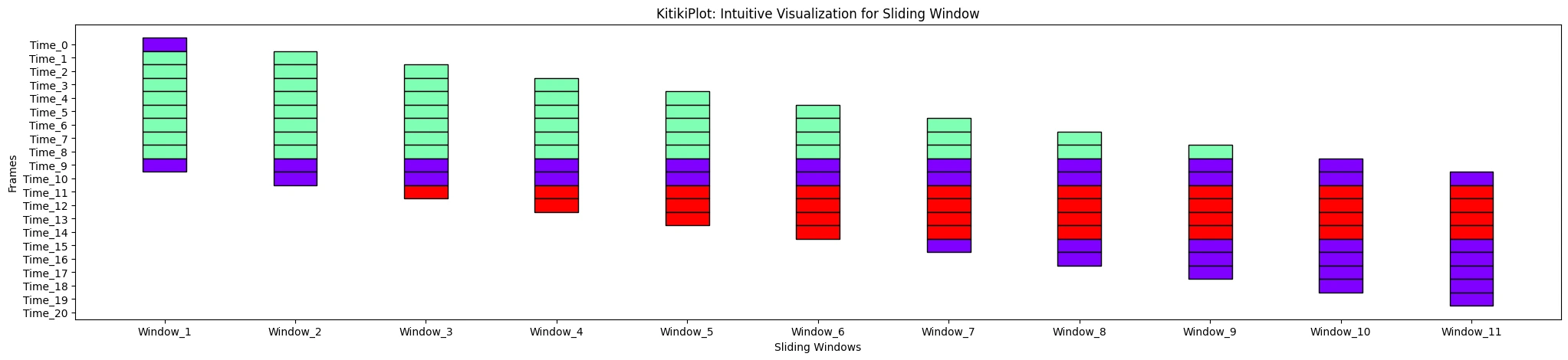

xticks_values : listing (elective)

• Checklist containing the values for xticks
• Default is []

ktk= KitikiPlot( knowledge= df["Summary"].values.tolist() )
xtick_values= ['Start', "T1", "T2", "T3", "T4", "T5", "T6", "T7", "T8", "T9", "End"]
ktk.plot( xticks_values= xtick_values )

yticks_values : listing (elective)

• Checklist containing the values for yticks
• Default is []

ktk= KitikiPlot( knowledge= df["Summary"].values.tolist() )

yticks_values= [(str(i.hour)+" "+i.strftime("%p").lower()) for i in  pd.to_datetime(df["Formatted Date"])]
ktk.plot( yticks_values= yticks_values )

xticks_rotation : int (elective)

• Rotation angle for x-axis tick labels.
• Default is 0.

ktk= KitikiPlot( knowledge= df["Summary"].values.tolist() )
ktk.plot( xticks_rotation= 45 )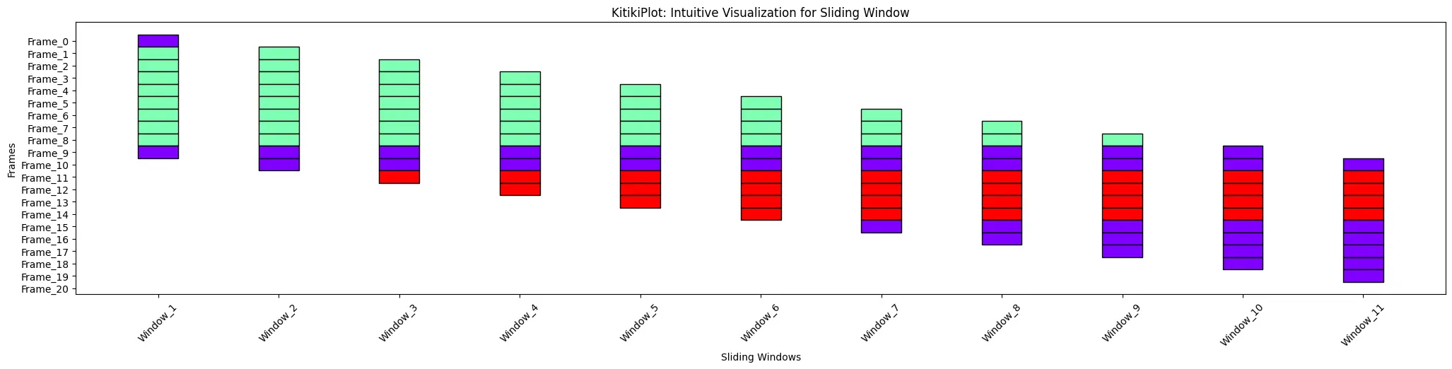

yticks_rotation : int (elective)

• Rotation angle for y-axis tick labels.
• Default is 0.

ktk= KitikiPlot( knowledge= df["Summary"].values.tolist() )

ktk.plot( figsize= (20, 8),     # Improve top of the plot for good visualization (right here)
          yticks_rotation= 45 
        )

title : str (elective)

• The title of the plot.
• Default is “KitikiPlot: Intuitive Visualization for Sliding Window”.

ktk= KitikiPlot( knowledge= df["Summary"].values.tolist() )
ktk.plot( title= "KitikiPlot for Climate Dataset")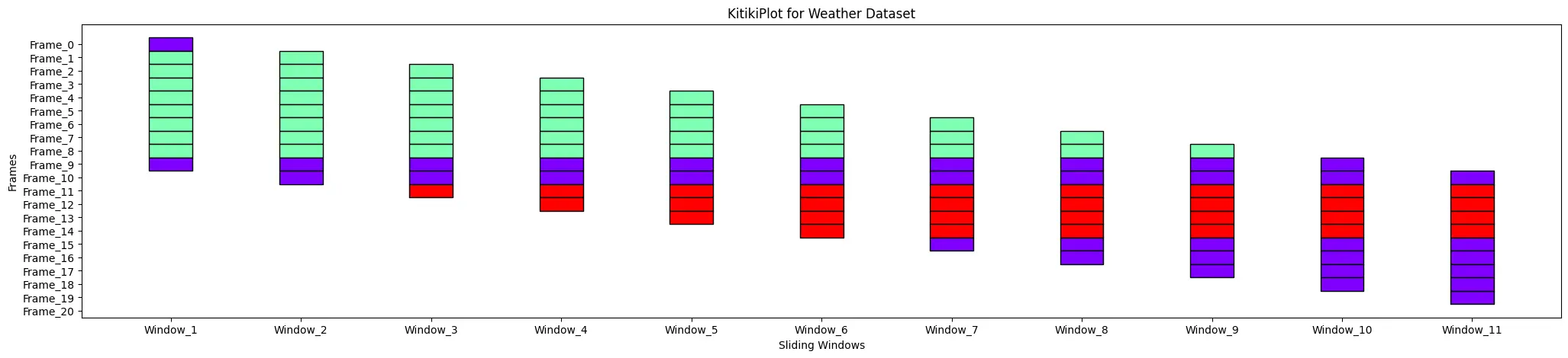

display_grid : bool (elective)

• A flag indicating whether or not to show grid on the plot.
• Default is False.

ktk= KitikiPlot( knowledge= df["Summary"].values.tolist()[:15] )
ktk.plot( display_grid= True )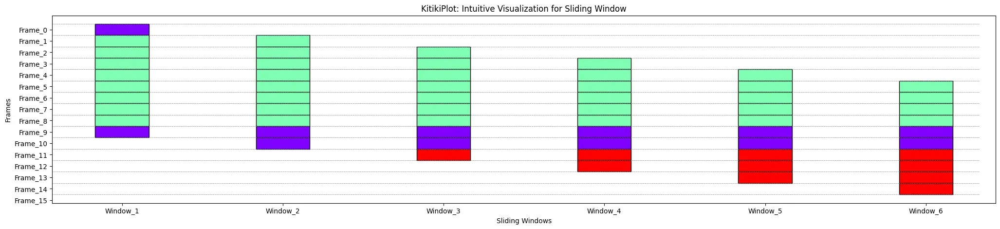

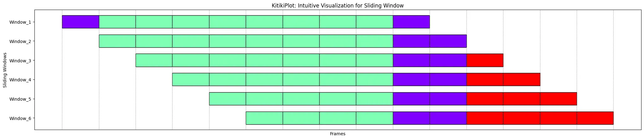
ktk= KitikiPlot( knowledge= df["Summary"].values.tolist()[:15] )

ktk.plot( 
          cell_width= 2,
          transpose= True,  
          xlabel= "Frames",
          ylabel= "Sliding Home windows",
          ytick_prefix= "Window",
          display_xticks= False,
          display_grid= True 
        )

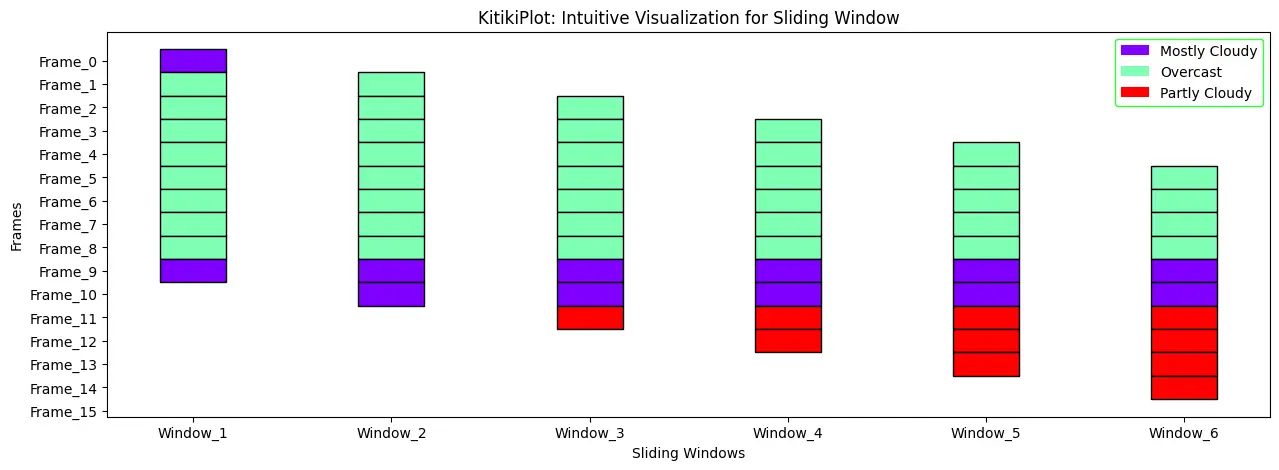
display_legend : bool (elective)

• A flag indicating whether or not to show a legend on the plot.
• Default is False.

ktk= KitikiPlot( knowledge= df["Summary"].values.tolist() )
ktk.plot( display_legend= True )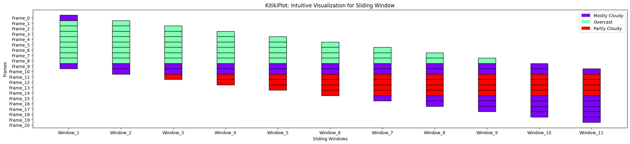

legend_hatch : bool (elective)

• A flag indicating whether or not to incorporate hatch patterns within the legend.
• Default is False.

ktk= KitikiPlot( knowledge= df["Summary"].values.tolist() )

ktk.plot( 
          cmap= {"Largely Cloudy": "#ffffff"},
          fallback_color= "white",
          display_hatch= True,
          display_legend= True,
          legend_hatch= True
        )

legend_kwargs : dict (elective)

• Further key phrase arguments handed to customise the legend.
• Default is {}.

Place legend outdoors of the Plot

ktk= KitikiPlot( knowledge= df["Summary"].values.tolist()[:15] )

ktk.plot( 
        figsize= (15, 5),
        display_legend= True,
        legend_kwargs= {"bbox_to_anchor": (1, 1.0), "loc":"higher left"} )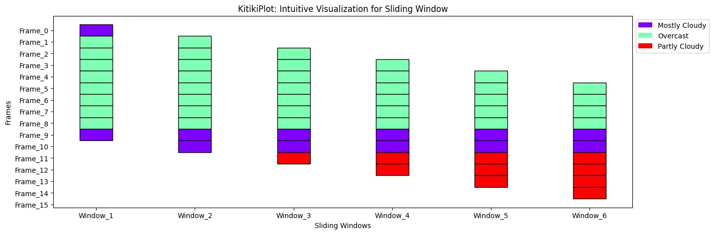

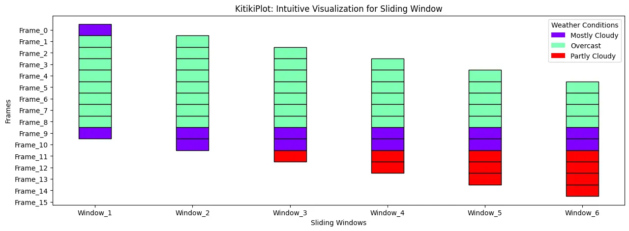
Set title for the legend————————————

ktk= KitikiPlot( knowledge= df["Summary"].values.tolist()[:15] )

ktk.plot( 
          figsize= (15, 5),
          display_legend= True,
          legend_kwargs= {"title": "Climate Situations"} 
        )

Change edgecolor of the legend

ktk= KitikiPlot( knowledge= df["Summary"].values.tolist()[:15] )

ktk.plot( 
          figsize= (15, 5),
          display_legend= True,
          legend_kwargs= {"edgecolor": "lime"} 
        )

kitiki_cell_kwargs : dict (elective)

• Further key phrase arguments handed to customise particular person cells.
• Default is {}.

Set the road fashion

ktk= KitikiPlot( knowledge= df["Summary"].values.tolist()[:15] )

ktk.plot( 
        figsize= (15, 5),
        kitiki_cell_kwargs= {"linestyle": "--"} )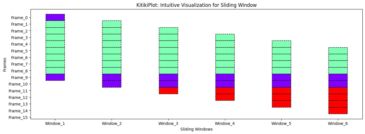

Alter the road width

ktk= KitikiPlot( knowledge= df["Summary"].values.tolist()[:15] )

ktk.plot( 
        figsize= (15, 5),
        kitiki_cell_kwargs= {"linewidth": 3} )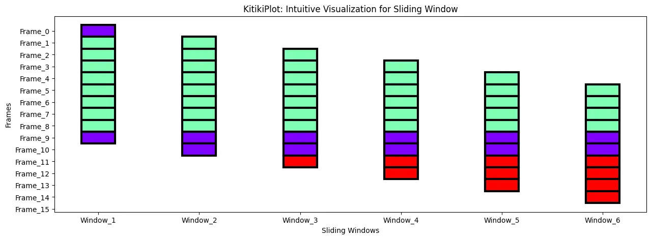

Alter the alpha

ktk= KitikiPlot( knowledge= df["Summary"].values.tolist()[:15] )

ktk.plot( 
        figsize= (15, 5),
        kitiki_cell_kwargs= {"alpha": 0.4} )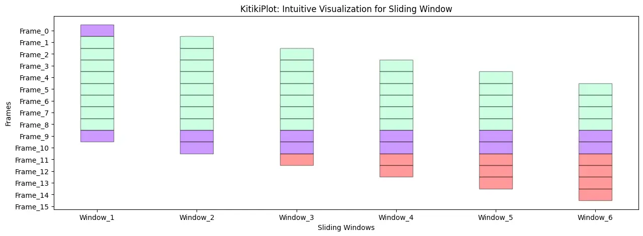

Actual-World Purposes of KitikiPlot

KitikiPlot excels in numerous fields the place knowledge visualization is essential to understanding complicated patterns and traits. From genomics and environmental monitoring to finance and predictive modeling, KitikiPlot empowers customers to remodel uncooked knowledge into clear, actionable insights. Whether or not you’re analyzing massive datasets, monitoring air high quality over time, or visualizing traits in inventory costs, KitikiPlot affords the flexibleness and customization wanted to fulfill the distinctive calls for of assorted industries.

Genomics

• KitikiPlot allows clear visualization of gene sequences, serving to researchers determine patterns and motifs.
• It facilitates the evaluation of structural variations in genomes, important for understanding genetic issues.
• By offering visible representations, it aids in deciphering complicated genomic knowledge, supporting developments in customized drugs.

Dataset URL: https://archive.ics.uci.edu/dataset/69/molecular+biology+splice+junction+gene+sequences

# Import crucial libraries
from kitikiplot import KitikiPlot
import pandas as pd

# Load the dataset
df= pd.read_csv( "datasets/molecular+biology+splice+junction+gene+sequences/splice.knowledge", header= None )

# Rename the columns
df.columns= ["Label", "Instance_Name", "Nucleotide_Sequence"]

# Choose 3 gene sequences randomly
df= df.pattern(3, random_state= 1)

# Take away the white areas from the "Nucleotide_Sequence"
df["Nucleotide_Sequence"]= df["Nucleotide_Sequence"].str.strip()

df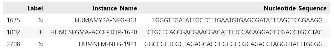

index= 0

ktk= KitikiPlot( knowledge= [i for i in df.iloc[index, 2]], stride= 1, window_length= len(df.iloc[index, 2]) )

ktk.plot(
        figsize= (20, 0.5),
        cell_width= 2,
        cmap= {'A': '#007FFF', 'T': "#fffc00", "G": "#00ff00", "C": "#960018"},
        transpose= True,
        xlabel= "Nucleotides",
        ylabel= "Sequence",
        display_yticks= False,
        xtick_prefix= "Nucleotide",
        xticks_rotation= 90,
        title= "Genome Visualization: "+df.iloc[index, 1].strip()+", Label : "+df.iloc[index,0].strip(),
        display_legend= True,
        legend_kwargs= {"bbox_to_anchor": (1.01, 1), "loc":'higher left', "borderaxespad": 0.})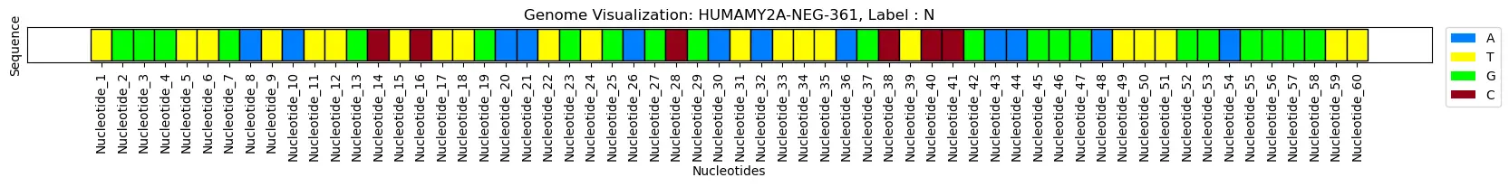

Climate Forecasting

• The library can successfully characterize temporal climate knowledge, reminiscent of temperature and humidity, over sequential time home windows to determine traits.
• This visualization aids in detecting patterns and fluctuations in climate situations, enhancing the accuracy of forecasts.
• Moreover, it helps the evaluation of historic knowledge, permitting for higher predictions and knowledgeable decision-making concerning weather-related actions.

Dataset URL: https://www.kaggle.com/datasets/muthuj7/weather-dataset

# Import crucial libraries
from kitikiplot import KitikiPlot
import pandas as pd

# Learn csv
df= pd.read_csv( "datasets/weatherHistory/weatherHistory.csv")
print("Form: ", df.form)

# Choose a subset of information for visualization
df= df.iloc[45:65, :]
print("Form: ", df.form)

df.head(3)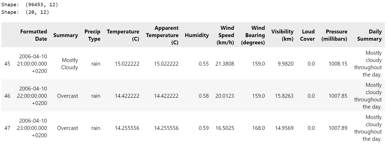

index= 0

weather_data= ['Mostly Cloudy', 'Overcast', 'Overcast', 'Overcast', 'Overcast', 'Overcast','Overcast', 'Overcast', 
               'Overcast', 'Mostly Cloudy', 'Mostly Cloudy', 'Partly Cloudy', 'Partly Cloudy', 'Partly Cloudy', 
               'Partly Cloudy', 'Mostly Cloudy', 'Mostly Cloudy', 'Mostly Cloudy', 'Mostly Cloudy', 'Mostly Cloudy']
time_period= ['21 pm', '22 pm', '23 pm', '0 am', '1 am', '2 am', '3 am', '4 am', '5 am', '6 am', '7 am', '8 am', 
              '9 am', '10 am', '11 am', '12 pm', '13 pm', '14 pm', '15 pm', '16 pm']
ktk= KitikiPlot( knowledge= weather_data, stride= 1, window_length= 10 )
ktk.plot(
        figsize= (20, 5),
        cell_width= 2,
        transpose= False,
        xlabel= "Window",
        ylabel= "Time",
        yticks_values= time_period,
        xticks_rotation= 90, 
        cmap= {"Largely Cloudy": "brown", "Partly Cloudy": "#a9cbe0","Overcast": "#fdbf6f"},
        legend_kwargs= {"bbox_to_anchor": (1.01, 1), "loc":'higher left', "borderaxespad": 0.},
        display_legend= True,
        title= "Climate Sample on 10-04-2006")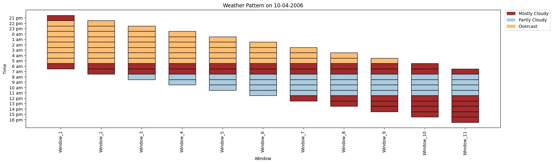

Air High quality Monitoring

• Customers can analyze pollutant ranges over time with KitikiPlot to detect variations and correlations in environmental knowledge.
• This functionality permits for the identification of traits in air high quality, facilitating a deeper understanding of how completely different pollution work together and fluctuate on account of numerous components.
• Moreover, it helps the exploration of temporal relationships between air high quality indices and particular pollution, enhancing the effectiveness of air high quality monitoring efforts.

Dataset URL: https://archive.ics.uci.edu/dataset/360/air+high quality

from kitikiplot import KitikiPlot
import pandas as pd

# Learn excel
df= pd.read_excel( "datasets/air+high quality/AirQualityUCI.xlsx" ) 

# Extract knowledge from at some point (2004-11-01)
df= df[ df['Date']== "2004-11-01" ]
print("Form : ", df.form)
df.head( 3 )

# Convert float to int
df["CO(GT)"]= df["CO(GT)"].astype(int)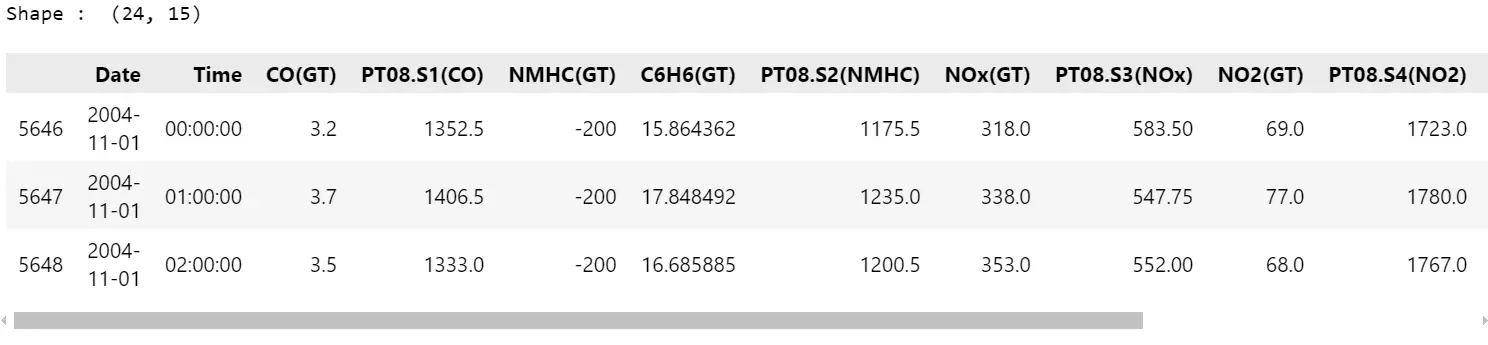

CO_values= [3, 3, 3, 3, -200, 2, 1, 1, 1, 1, 2, 3, 4, 4, 3, 3, 3, 2]
time_period= ['0 am', '1 am', '2 am', '3 am', '4 am', '5 am', '6 am', '7 am', '8 am', '9 am', '10 am',
              '11 am', '12 pm', '13 pm', '14 pm', '15 pm', '16 pm', '17 pm']
ktk= KitikiPlot( knowledge= CO_values )
ktk.plot(
        figsize= (20, 5),
        cell_width= 2,
        cmap= {-200: "cornflowerblue", 1: "#ffeaea", 2: "#feb9b9", 3: "#ff7070", 4: "#b00"},
        transpose= True,
        xlabel= "Time",
        ylabel= "Sliding Home windows of CO(GT) values (in mg/m^3)",
        display_xticks= True,
        xticks_values= time_period,
        ytick_prefix= "Window",
        xticks_rotation= 90, 
        display_legend= True,
        title= "CO(GT) Pattern in Air",
        legend_kwargs= {"bbox_to_anchor": (1.01, 1), "loc":'higher left', "borderaxespad": 0.})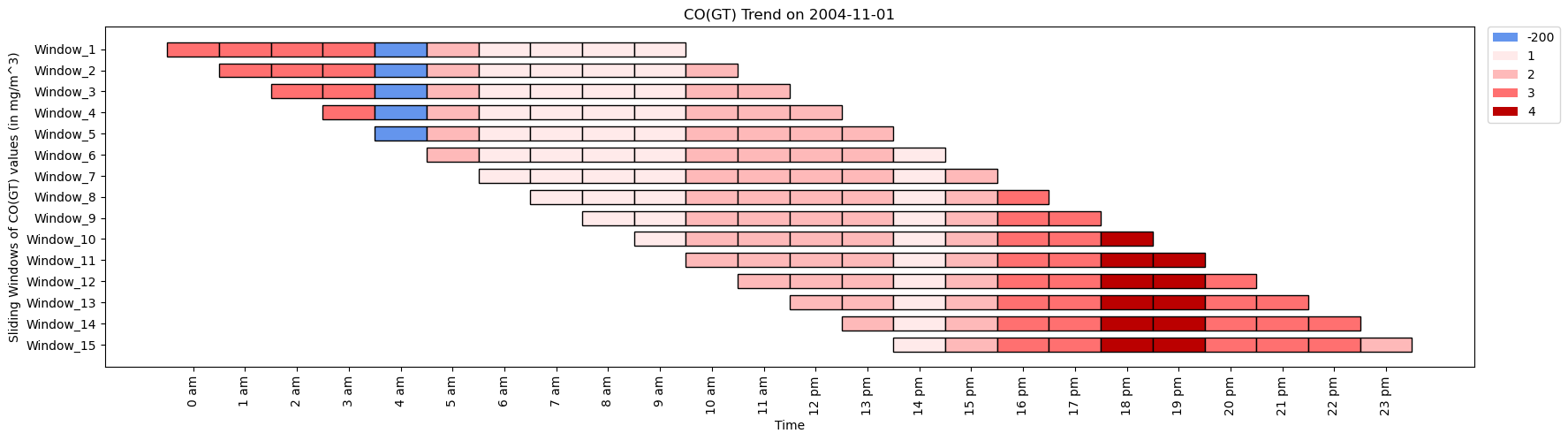

Conclusion

KitikiPlot simplifies the visualization of sequential and time-series categorical sliding window knowledge, making complicated patterns extra interpretable. Its versatility spans numerous functions, together with genomics, climate evaluation, and air high quality monitoring, highlighting its broad utility in each analysis and trade. With a concentrate on readability and value, KitikiPlot enhances the extraction of actionable insights from categorical knowledge. As an open-source library, it empowers knowledge scientists and researchers to successfully sort out numerous challenges. 

Key Takeaways

• KitikiPlot is a flexible Python library designed for exact and user-friendly sliding window knowledge visualizations.
• Its customizable parameters enable customers to create significant and interpretable visualizations tailor-made to their datasets.
• The library helps a variety of real-world functions throughout numerous analysis and trade domains.
• As an open-source instrument, KitikiPlot ensures accessibility for knowledge science practitioners and researchers alike.
• Clear and insightful visualizations facilitate the identification of traits in sequential categorical knowledge.

Sources

Quotation

@software program{ KitikiPlot_2024
writer = {Boddu Sri Pavan and Boddu Swathi Sree},
title = {{KitikiPlot: A Python library to visualise categorical sliding window knowledge}},
12 months = {2024},
model = {0.1.2},
url = {url{https://github.com/BodduSriPavan-111/kitikiplot},
doi = {10.5281/zenodo.14293030}
howpublished = {url{https://github.com/BodduSriPavan-111/kitikiplot}}
}

Steadily Requested Questions

The media proven on this article will not be owned by Analytics Vidhya and is used on the Writer’s discretion.